Regression Models for AirBnB Price Prediction in San Diego
Airbnb Incorporated is a software company that enables individuals to rent out their private residences or properties to individuals through their app and website, allowing users to generate residual income off their unused real estate assets. Since it’s conception in 2007, and its initial public offering in 2020, Airbnb has amassed a market cap exceeding $329B, effectively accounting for over 5% of the Travel Services industry (Yahoo Finance). Pricing for Airbnb rentals are determined solely by the individual owners of the residence, and their respective outlook on the property value, the geographical location’s viability as a tourist destination, and the host’s required rate of return. This study intends to train a machine learning model to predict the price of Airbnb listings in the San Diego Metropolitan area based upon the listing’s geographic location, accommodation capacity, and amenities
Key Findings
This study found that a Support Vector Regression (SVR) and Random Forest (RF) model was successful in predicting San Diego Airbnb pricing up to 70% based upon the listing’s geographic location, accommodation capacity, and amenities.
Data Sources
Data for this analysis was obtained through Inside Airbnb a public data repository offering AirBnB listing data for a variety of geographical locations. This platform offered a San Diego specific dataset which was used for this study.
This dataset had nearly 30 features, including a number of important elements in determining pricing such as bedroom and bathroom number, ratings, and listing location.
Data Cleaning and Preliminary Statistics
Data from Inside Airbnb was received in a .csv format, typical for tabular data. However an initial roadblock that was encountered was ensuring the data received was in good format. Out of the gate, key features such as bedroom, bathroom, and bed number were all in a single column, delimited with a common symbol. Excel's Text to Columns was utilized to split the data into their own respective columns like so:
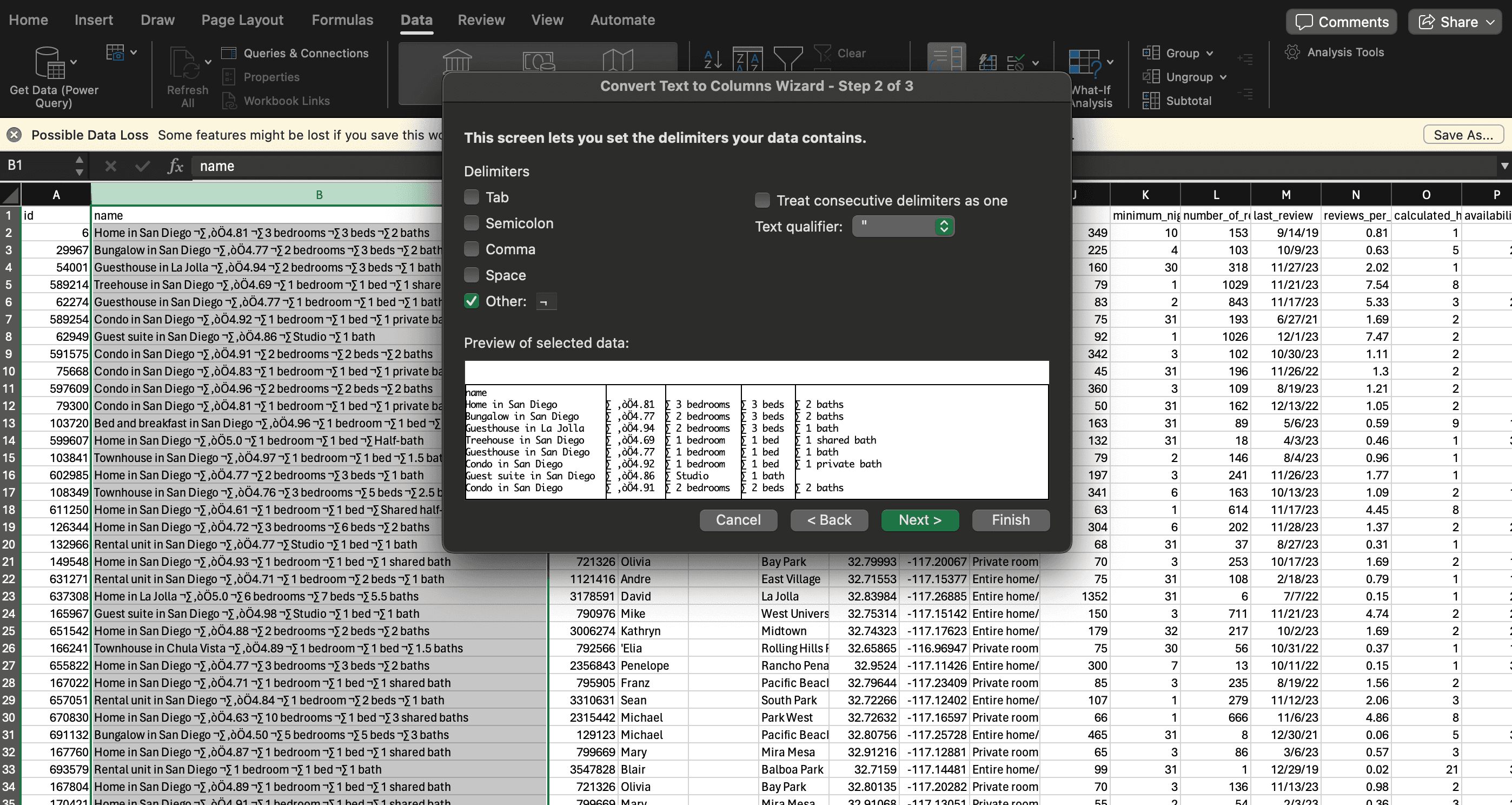
Once the data was divided into their respective columns, out of place symbols were removed using Excel's Find & Replace. The next issue that arose, however, was that not all listings had bedroom, bathroom, and bed information. For some, the bedroom value existed but not the bed, and vice versa. Due to this, the initial excel data split resulted in inconsistent formatting, where values would be in incorrect columns. To solve this, the .csv data was read into a Pandas DataFrame where it was iterated through programmatically, and placed into the correct column (rating, bedroom, bathroom, or bed) based on the text content of the specific cell.
for index, row in df.iterrows():
    # iterate through keywords, if they match, assign to the correct column
    rating = None
    bedroom = None
    bed = None
    bathroom = None

    # check if rating is a number
    try:
        rating = float(str(row['rating']).strip())
    except ValueError:
        if 'New' in str(row['rating']):
            rating = row['rating']
    else:
        if not bedroom and 'bedroom' in str(row['rating']) or 'Studio' in str(row['rating']):
            bedroom = row['rating']
        elif not bathroom and 'bath' in str(row['rating']):
            bathroom = row['rating']
        elif not bed and 'bed' in str(row['rating']) and (not 'bedroom' in str(row['rating']) or not 'Studio' in str(row['rating'])):
            bed = row['rating']

    # Same logic for bedroom, bed, and bathroom number...

    # assign correct values to columns
    df.loc[index, 'rating'] = rating
    df.loc[index, 'bedroom'] = bedroom
    df.loc[index, 'bed'] = bed
    df.loc[index, 'bath'] = bathroom
Now that the values, corresponded to the correct columns, the numerical value of each of the derived columns (bedroom, bathroom, bed) were extracted using NumPy, a popular python statistic library. Additionally, unique values were handled such as "New" in the ratings column, or "Studio" in the bedroom column, which required a little extra leg work to ensure data formatting was accurate.
# Account for unique values
for index, row in df.iterrows():
    if 'New ' in str(row['rating']):
        row['rating'] = 0
    if 'Studio' in str(row['bedroom']):
        row['bedroom'] = 1

# Bed/Bedroom Formatting
df['bedroom'] = np.where(df['bedroom'] == 'Studio ', 1, df['bedroom'])
df['bed_num'] = df['bed'].str.extract('(\d+)').astype(float)
df['bedroom_num'] = df['bedroom'].str.extract('(\d+)').astype(float)
# Bathroom Formatting
df['bath'] = np.where(df['bath'] == 'Half-bath', 0.5, df['bath'])
df['bath'] = np.where(df['bath'] == 'Shared half-bath', 0.5, df['bath'])
df['bath_num'] = df['bath'].str.extract('(\d+)').astype(float)
# Rating Formatting
df['rating'] = np.where(df['rating'] == 'New ', 0, df['rating'])
Finally, the text-based columns for these fields, as well as a couple different data features were dropped. Finally, any remaining records with NA values were dropped. This resulted in a cleaned dataset of just under 9000 records, ready to be used in our predictive models.
Preliminary Statistics and Visualizations
Some basic statistics were derived from the dataset were calculated using Pandas, including the mean and median number of bedrooms, bathrooms, and beds, as well as the average and median nightly price for all listings.
- Bedrooms - Mean: 2.05, Median: 2
- Beds - Mean: 2.91, Median: 2
- Bathrooms - Mean: 1.59, Median: 1
- Nightly Price - Mean: 268.36, Median: 170.5
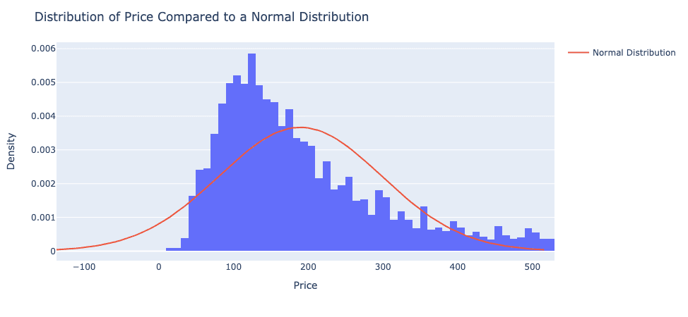
From these statistics, we can safely assume that the median AirBnB in San Diego has 2 beds, 1 bath, and costs about $170 a night. One can also recognize that the price distribution is positively skewed, as the mean is much higher than the median and observed in the graph below.
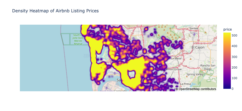
A unique variable in real estate, and especially AirBnB listings, is the location of the listing. Especially in an area with prominent coastal real estate like San Diego, small homes could still drive very steep nightly prices due to their location. A heatmap was employed to visualize the effect of this, and the relationship between coastal proximity and nightly price is obvious.
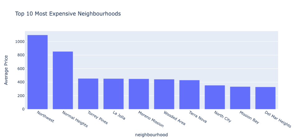
Additionally, average price per neighbourhood was calculated and graphed to determine the San Diego neighbourhoods that contained the most expensive listings, unsuprisingly, many coastal neighbourhoods made an appearance in the top 10.
Model Construction and Fine Tuning
Now that there was an understanding of the dataset, it was time to create and train the models. Many machine learning models in the SciKitLearn library require only numerical data. As aforementioned, our dataset includes categorial data fields, such as neighbourhood and room type that likely have influence on the final price of the listing. To be able to include this our test set, SciKitLearn's label encoder was used to convert the categorical room type and neighbourhood variables into a numerical representation. Now, these variables could be used by our models and the categorical columns can be dropped.
from sklearn.preprocessing import LabelEncoder

# Create a LabelEncoder instance
label_encoder = LabelEncoder()

# Fit the LabelEncoder to the concatenated Series of all categorical variables
label_encoder.fit(pd.concat([df['neighbourhood'], df['room_type']]))
# Transform each categorical variable into numerical form
df['neighbourhood_encoded'] = label_encoder.transform(df['neighbourhood'])
df['room_type_encoded'] = label_encoder.transform(df['room_type'])
Model parameters were fine tuned using Grid Search. Grid search is an exhaustive search over specified parameter values for an estimator. The method implements the fit and score methods. The parameters of the estimator used to apply these methods are optimized by cross validated grid search over the parameter grid. In short, common parameter values are outlined and then iterated through to determine which parameter combinations produce the most accurate results. The code below shows the process of splitting the dataset, training a Random Forest Model using the optimized parameters, and calculating accuracy metrics such as MAPE, MAE, and residuals.
X = df.drop(columns=['price'])  # Features
y = df['price']  # Target variable

# Splitting the dataset into the training set and test set
X_train, X_test, y_train, y_test = train_test_split(X, y, test_size=0.2, random_state=42)

# Initialize RandomForestRegressor model
rf_model = RandomForestRegressor(max_depth=30, min_samples_leaf=2, min_samples_split=5)
rf_model.fit(X_train, y_train)
y_pred = rf_model.predict(X_test)

# Calculate Metrics
mae = mean_absolute_error(y_test, y_pred)
mape = mean_absolute_percentage_error(y_test, y_pred)
residuals = y_test - y_pred
Initial Model Results
Initial model results were largely inconclusive with High MAPEs and MAEs. The graph below shows the prediction of the Random Forest Regressor. Notice certain extreme outliers in the dataset.
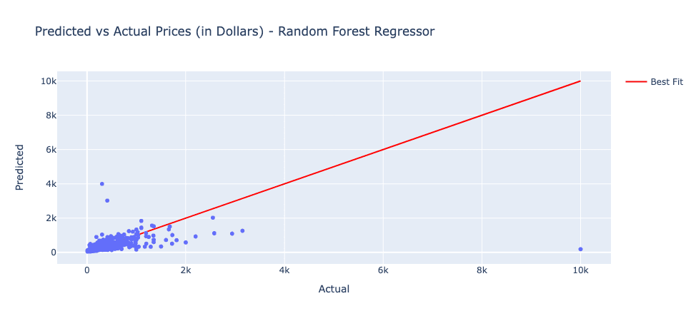
In an effort to improve model results, a couple measures were taken. First, outliers were removed from the dataset using an interquartile range in the code below.
# Calculate IQR
Q1 = df['price'].quantile(0.25)
Q3 = df['price'].quantile(0.75)
IQR = Q3 - Q1
# Filter out outliers
df = df[(df['price'] >= (Q1 - 1.5 * IQR)) & (df['price'] <= (Q3 + 1.5 * IQR))]
Then the feature set the models were trained on was paired down in an effort to not introduce variables that had little effect on the final price. The output below shows the structure of the training set of the most successful models. As you can see, only 7 features of the nearly 30 initial features made it to the final training set.
<class 'pandas.core.frame.DataFrame'>
Index: 8217 entries, 6 to 1031339997516779049
Data columns (total 8 columns):
 #   Column                 Non-Null Count  Dtype
---  ------                 --------------  -----
 0   latitude               8217 non-null   float64
 1   longitude              8217 non-null   float64
 2   price                  8217 non-null   int64
 3   bed_num                8217 non-null   float64
 4   bedroom_num            8217 non-null   float64
 5   bath_num               8217 non-null   float64
 6   neighbourhood_encoded  8217 non-null   int64
 7   room_type_encoded      8217 non-null   int64
dtypes: float64(5), int64(3)
memory usage: 577.8 KB
Final Model Results
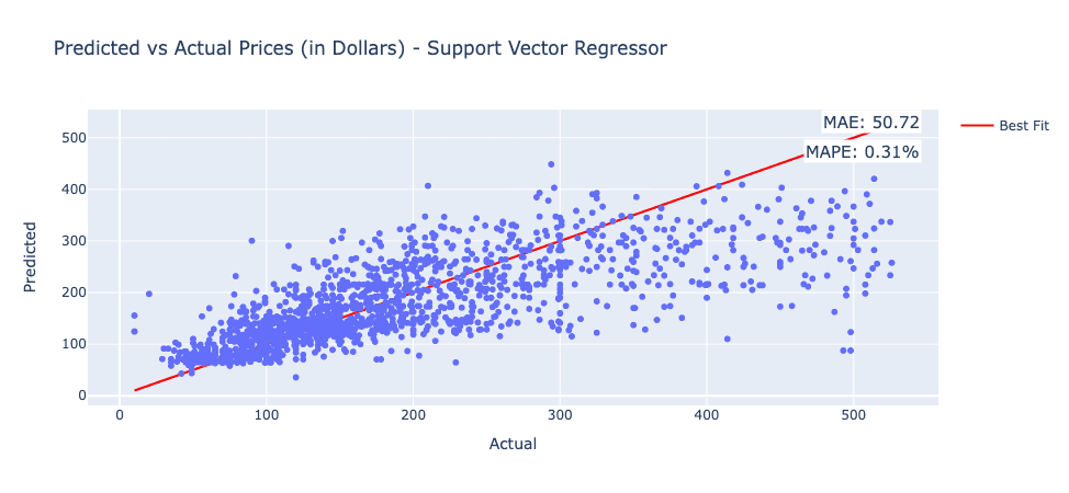
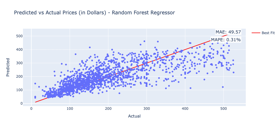
After filtering out the outliers and pairing down the feature set, models showed much more promising results. Both models ended with very similar accuracy metrics.
Support Vector Regression
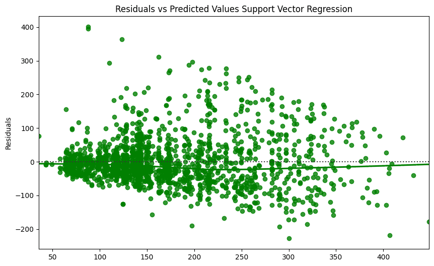
The graphs below show the Predicted vs. Actual Performance of the SVR model. The SVR Model recorded an MAE of 50.72 and a MAPE of 0.308%.
Random Forest Regressor
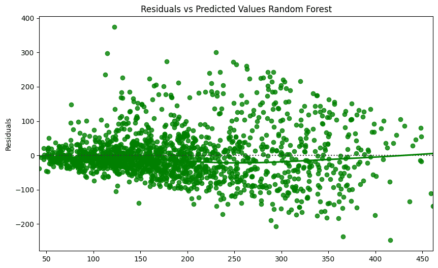
The graphs below show the Predicted vs. Actual Performance of the RF model. The RF Model recorded an MAE of 49.57 and a MAPE of 0.305%.
Discussion and Future Work
As observed in the results, both models were reasonably accurate in their predictions, but based upon the residual graph, underestimated the prices of most homes. Nevertheless, both models recorded very similar accuracy metrics, possibly alluding to the difficulties in prediction of this dataset. Predicting AirBnB nightly prices proved to be a challenging task, and machine learning models appear to be moderately accurate in their forecasting. Further fine tuning and examining different areas of study might produce more accurate results.
These findings could be applied to additional research as well as AirBnB hosts in the San Diego Metropolitan area. Accurate models could be used by hosts to accurately price their listing in accordance with the trends of the area to maximize revenue and booking.
A potential limitation of this study is the variability in AirBnB pricing despite similar accommodations and locations. This may be due to the innate human involvement in pricing decisions. For example, individuals who rent out their primary residence may be more prone to charge higher than individuals or companies who rent out their additional properties. Further research on the effects of human psychology on their pricing decisions would be an interesting continuation of this study.
Conclusion
The Support Vector Regression and Random Forest Model both recorded 70% accuracy respectively in prediction of AirBnB prices in the San Diego Metropolitan area. These findings suggest that there may be some viability in machine learning price predictors for AirBnB hosts to accurately price their listings to be aligned with current market trends.